Copyright Notice: This article is Copyright AI Factory Ltd. Ideas and code belonging to AI Factory may only be used with the direct written permission of AI Factory Ltd.
This topic is an indulgence. It explores low-level tricks to achieve significant speed-ups in code, focusing on methods with limited theoretical grounding. These tricks provide rapid results by emulating processes that are otherwise very slow.
Why do this?
When we started in the games industry, the game devices were slow, yet the demands of the games were very high. Although the need for optimisation is diminishing as game devices become faster, the sometimes oddball craft required for this is worth documenting for future instances when performance must be maximized to meet some overwhelming requirement. Back in the '80s, every machine cycle was gold, and even just 15 years ago, performance was a critical factor for many games. It's also important to note that early microprocessors lacked floating-point support, so it became standard practice to map requirements to fit integer implementations. The inclination to do this is hard to shake off, and I often find myself using integers where I could use floats.
In this article, we present two examples: one from a recent project and another from 16 years ago. These methods were necessary at the time and represent a type of craft that may soon disappear. The second example, previously published, was sufficiently vital and innovative that it deserves a re-airing. It also replaced an ad hoc approach with a systematic method for creating the needed code.
(1) Backgammon
Determining When We Know We May Win
Our Backgammon program needs to make a probability decision before each CPU dice throw, determining whether or not to offer a double. This is a non-trivial decision, as it requires assessing the probability of winning from the current position. If the chances are better than even, the program can offer to double the points for that round, allowing the winning player to earn double points. At that point, the opponent can choose to refuse the double and fold, giving the opponent N points instead of risking giving them 2xN points.

In the original version of Backgammon published in 2010, a linear evaluation was used to estimate whether the program was likely to win. This task is not straightforward, and only after extensive testing against multiple playouts did it become clear that the linear evaluation was not performing well. This doesn't necessarily indicate a significant flaw in the evaluation itself, but rather highlights how challenging it is to estimate a final game outcome using a static evaluation of the current position. Note that this is much more difficult than it would be in a game like chess, where a simple material tally can give a good indication of the likely outcome. In Backgammon, not only is there no simple measure like that, but the outcome also depends on the unpredictable fortune of future dice rolls.
The solution was to play out the game from the current position to determine the likely winner. Again, in chess, this might be resolved by playing out just a few sample games, since each playout faces the same circumstances. In Backgammon, however, many more games need to be played out, as each playout involves different dice rolls. Therefore, you are making a probability decision influenced by the randomness of the dice.
An implementation that might follow this approach could involve the program playing a fixed number of games, then examining the win rate to decide whether a win is likely. However, this method has the following sequential flaws:
| 1. | How do you determine how many wins are needed to be confident that a win is more probable? A simple majority may not be sufficient. Achieving confidence with a simple majority might require an impractically large number of games. | ||
| 2. | To address the issue above, you can use a binomial distribution to calculate how many wins are necessary. If you require 95% confidence that a win is more probable, then in 100 rollouts, you would need to win 58 games. | ||
| 3. | Playing 100 games is time-consuming and will cause a noticeable pause each time the CPU takes a turn to throw its dice. This significant delay is problematic. | ||
The solution is to keep playing games until the win/loss rate gives us 95% confidence that a win is more likely. While this approach isn't entirely sound (as it risks selecting the sample that provides the desired outcome), it still holds validity. This allows successive rollouts to continue until the threshold is reached, and also permits early termination if the results indicate a high probability of losing. This approach is effective because the 100-game target can often be aborted very early, either because there are enough wins to be confident of victory or enough losses to know it's a lost cause. This optimised solution can reduce the number of games tested to as few as 10, so the player generally won't notice a fixed pause before each dice roll. A perceptive player might notice a slight delay when the situation is evenly matched, but this makes the program appear to behave more human-like, hesitating when faced with uncertainty.
The above is already an optimised way of assessing this, but the special optimisation follows here:
Providing access to the Binomial Distribution
To estimate whether the result satisfies the 95% confidence level, the calculation of many binomial terms is required, which involves extensive floating-point math. For a fixed number of games, this could be pre-calculated into a table. However, since we do not know how many games will be played, we would need tables for each possible number of target games. This is not ideal.
We have a workaround that addresses this issue. Ideally, we wanted a simple formula that approximates the conclusion of the binomial distribution. While that might not sound feasible, it can be achieved within acceptable margins of error.
Procedure for Devising a Fast Formula
This is where spreadsheets become valuable. You can set up a table that covers the full range of possible games that might be played, capped at 100 in this case. Then, using the binomial theorem, you can find the closest approximation to 95% confidence for a few sample points within the range of 1 to 100 games. In practice, it was expected that mostly the lower range of games would be used, between 10 and 30 games, so more sample points were calculated in that range. For example, for 10 games, the nearest match to 95% confidence is 8 wins and 2 losses, giving 96.70%. Further down the table, with 30 games, the best fit is 20 wins and 10 losses, giving 94.49%.
The procedure then is to create a formula that seems to mimic these values and apply it to all cells in the range of 1 to 100 games (in practice, this range was 10 to 100, in steps of 2, based on the assumption that if the formula works well for 30 and 32 games, it will likely be accurate for 31 as well). Such a formula is likely to be parameterised, so these cells duplicated a formula that referenced a shared table.
From there, you experiment with a few simple linear terms to see which ones appear to reproduce the number of wins needed to satisfy the 95% confidence level. As the formula improved, more reference target values were added to the table to fine-tune it. The resulting formula was:
| Wins = 2+INT(num*4/5)-INT((num+1)/(5)) | where "num" is the number of games played |
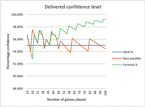
Note that this formula at various points will create rounding spikes, as it uses integers. If we look at how accurate this was we can see a plot of:
| 1. | The perfect goal of 95% | |
| 2. | The best possible given the integer limits imposed by a limit number of games, and | |
| 3. | The final formula calculated value. |
This is plotted only for even numbers of games, but odd numbered numbers of games would still be expected to deliver within the same bounds.

From this, you can see that the best possible outcome does deviate from the ideal 95%, as it must, due to the limited granularity imposed by the number of games played. However, the formula matches the best possible result most of the time in the range of 10 to 46 games, but thereafter deviates, delivering a confidence bound that rises from 97.10% to a maximum of 99.17% after 100 games.
Is this acceptable? Yes, it is, because in practice, almost all of the time, no more than 30 games are played, and most of the time, fewer than 20 games are played. The formula within this low range is nearly spot-on to the best possible outcome, and later on, it deviates to require a higher confidence bound, still only reaching 98% after 60 games.
This is not an actuarial calculation but one intended for use in a game to ensure that offers of doubles have a reasonable level of confidence that they are correct. This running formula allows the program to dynamically abort searches when the confidence bounds indicate that more searches are unlikely to change the decision from no double offer to a double offer.
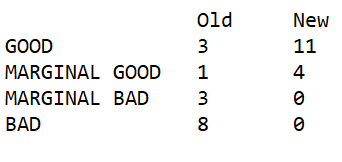
It is extremely fast and compact, with no need for a more accurate or elaborate solution. The performance of this new doubling code can be seen in the table below, which compares the performance of the old doubling offer code and the new doubling offer code. I classified the outcomes as BAD where a double was not offered when it should have been. In no instances was a double offered when it should not have been. This was compared against many full rollouts from many positions to determine the chance of winning. From this, the new code performs very well, but the old code misses many doubling opportunities.

(2) Optimising Collision Detection in an Aquarium Simulation
This optimisation was detailed at length in our first article in 2006, in relation to an aquarium project. I initially planned to simply reference this example here, but the original article is detailed and lengthy, so it's better to provide a preamble and summary, with a link to that article.
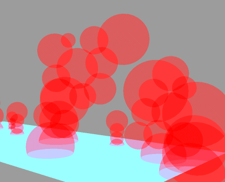
The problem involves avoiding collisions between objects in an aquarium simulation, running on a slow mobile phone without hardware floating-point support. Mapping collisions between actual 3D models was not feasible, so instead, objects were approximated using a limited number of spheres in the 3D space. This approach reduced collision detection to checking for intersections between these spheres. A single fish might be represented by three or more spheres, while a rock or plant could have many more. Given that any tank might contain many fish, the number of potential collisions to consider could be substantial. The image below shows the distribution of collision spheres in one sample tank.

This process needed to be executed to detect collisions for all candidate objects about 20 times per second. Of course, some simple checks were always possible, such as detecting whether the difference in X, Y, or Z coordinates exceeded the sum of the radii of the two spheres. This allowed many potential collisions to be immediately rejected. However, when overlap was possible, a much more complex and computationally expensive test was required.
Consider the formula for calculating the distance between just two spheres:
Dist = SQRT(diffX*diffX + diffY*diffY + diffZ*diffZ)
Square root is not a standard processor instruction and must instead be solved using an iterative process, such as Newton's approximation, which involves looping through the expensive division instruction.
The full solution is provided in detail in the article Optimised Navigation of Complex 3D Worlds. The following is a shorter summary and further observation.
Essentially, this approach takes advantage of the fact that the distance between any two vectors varies between 1 and sqrt(2), or 1 and 1.414. The crude calculation of distance = X +Y/2 gives a range 1 to 1.5, which is a roughly similar value. This was the starting point, allowing delivery of a first approximation as follows:
x+(y>>1)+(z>>2)-(y>>3)-(z>>4)-(y>>5)-(z>>6)
This uses the operator >> which is shift right, or divide 2 power N.
This was expanded to add many similar random terms and these run through a long randomised test to detect the best approximation compared to SQRT(diffX*diffX + diffY*diffY + diffZ*diffZ).
This really worked and the following dropped out:
dist = x+(y>>1)-(y>>4)-(y>>5)+(z>>2)-(z>>7)-(z>>9)+(x>>7)-(x>>3)-(x>>9);
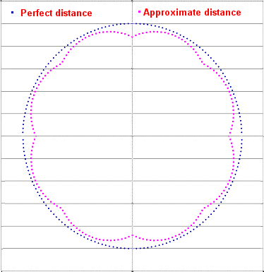
The efficacy of this can be demonstrated by the following plot, which compares the SQRT formula with the very fast approximation above.

From the above, it can be seen that the vector approximation maps quite well to the exact calculation. This level of approximation is entirely acceptable because the use of spheres in the first place is already a much larger approximation, as fish are not composed of merged spheres. The sphere mapping introduces a higher degree of error than the vector mapping described above.
On the development hardware, which by today's standards would be considered ancient (the Pentium 4 processor), this method achieved an 18-fold speed-up. Given that mobile phone hardware lacked floating-point capabilities, it's not hard to imagine a 100-fold speed-up on those devices.
This innovation had a profound impact on the program's design. It provided significant flexibility in checking for collisions, resulting in an aquarium simulation that allowed for much greater subtlety and delivered a highly realistic emulation.
Jeff Rollason - August 2024
