Copyright Notice: All code and ideas expressed in this article, are Copyright AI Factory Ltd.
You may use these, only with the direct written permission of AI Factory Ltd.
Modern gaming is seeing an expansion in game complexity. One manifestation of this is the desire to represent large complex 3D worlds. While advancing graphics hardware has been rapidly driving this forwards, processor speeds have not really kept pace. This shortfall means that game AI and physics has to work harder to keep up. Just because the graphics hardware might now be able to handle quadruple the number of rendered objects, the AI might not, supported by a more modest CPU resource advance.
This is a problem which we have had to consider, aggravated further by some processor hardware that is taking us in the opposite direction. In particular 3D hardware is now migrating to small devices such as PDAs and mobile phones, with processors that might not even have divide instructions, but are hooked up to an advanced 3D graphics processor.
Handling 3D space
Game programmers are well aware of the engineering needed to handle navigation and route finding in 2D space. When this is scaled up to handling 3D then the process of determining your position becomes more complex. A 2D route-finder might be supported by a 2D world represented by a 2D array to define where everything is. In 3D this technique is less attractive, for obvious reasons, so the programmer may instead need to define a hardwired 3D node map. The latter is generally not dynamic, so only works very well with fixed 3D worlds. Add to this that you might now consider the object navigating not as a point, but an object with multiple contact points, this does not help a 3D node map solver, as not all objects can reach all points. Given that an object may rotate, its effective shape may change, and that space may be filled by other blocking moving entities, then pre-calculated routes may not help. Given this it may be necessary to have a means of easily dynamically determining your position and projecting your expected position. Therefore it becomes imperative to be able to easily determine your location.
The Core: Calculating the distance between two points
The math required for is simple, but expensive. The distance between two points can be calculated by
Dist = SQRT(diffX*diffX + diffY*diffY + diffZ*diffZ)
Square root is not yet a conventional processor instruction, but instead needs solving in an instruction loop, such as Newtons approximation, which loops the expensive divide instruction..
Since vector distance is central to analysing 3D space, this is a key operation to try and optimise:
Faster Vector Arithmetic
Ideally you want to avoid long code calculations and slow instructions. If you examine vector calculations in 2D, you may notice that the vector length in 2D can be very approximately represented using some cheap maths, as follows:
Given X length 1 and Y length 0 to 1, then the vector between these varies between 1 and sqrt(2), that is 1 to 1.414. The trivial math X+Y/2 gives the range 1 to 1.5, a crude approximation to the above. If you refine this further to:
Dist = X +Y/2 Y/16 giving 1 to 1.4375
This is quite good, giving an error of just 1.6% for Y=1 down to 0% with Y=0.
An attractive aspect of this is that it uses only add and shift instructions, no divide. Divide by powers of 2 can be replaced by the very fast shift right instruction.
Experimenting with this further, converting to C++, and extending to 3D, we find that the following works:
x+(y>>1)+(z>>2)-(y>>3)-(z>>4)-(y>>5)-(z>>6)
>> is shift right here. >>4 is shift right by 4, or the equivalent of divide by 16.
This curious equation shifts by 1,2,3,4,5,6 in succession, yielding a calculation which has an average error of 1% and maximum of 12.4%. Of course the vector differences x,y and z have to be sorted into difference order, so that x is the largest difference.
Practical use of this fast method
Although this is quick, it has the property of both underestimating and overestimating vector distances. The consequence of the latter may result in a game object being in collision with another, as the vector calculation overestimates the distance. This may seem tolerable until you consider how it might be used, as follows:

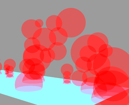
In this example, region in the 3D space is defined by overlapping bounding spheres. This is not exact, but allows a complex 3D object, composed of thousands of polygons, to be replaced by a modest number of bounding spheres. It will confine some space that is not actually bound by the objects, but can be arranged to ensure that no two objects can be allowed to overlap.
Consider the below for a scene of very high complexity:

This is a photo (of course) not a real 3D model, but if it was you can see that a scene might be filled with very complex objects, but represented to the AI by relatively few bounding spheres. The AI is thus freed from dealing with the full complexity of the scene.
Snags
Using this method will make use of a variety of bounding sphere sizes, including very large ones for representing surfaces, such as the ground. The snag here is that the absolute error in the vector calculation is in proportion to the bounding sphere size. If the bounding sphere is very large, then an overestimate of distance may result in a collision, or even an object becoming swallowed by another.
Refining the approximation
On the basis that underestimates of distances are acceptable, but overestimates are not, we need a new formula that guarantees never to overestimate distance.
The math behind our equation above is based on simple observation of the values of the numbers, rather than a theoretical model. Our solution for finding a refined formula was to get the program to create this formula for us, using experimentation. The program randomly generated formulae and tested these. As soon as it failed, another was tried. From testing hundreds of thousands of candidate formulae, the best one is the one which minimises the error, while guaranteeing no overestimates.
The result was the following:
dist = x+(y>>1)-(y>>4)-(y>>5)+(z>>2)-(z>>7)-(z>>9)+(x>>7)-(x>>3)-(x>>9);
with a worst-case of 12.4% underestimate and average error of 1.03%
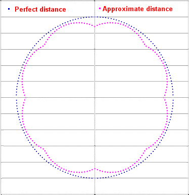
This is hard to visualise, but taking one cross-section of this we can see the following profile

From the above we can see that our bounding sphere is a lumpy sphere, but still a moderately good approximation.
Performance?
This needs the whole code to support it, as follows:
Comparing this to the conventional formula, using square root, it provides a speed-up of 18 times on an Althon64 and similar value on a Pentium 4. These are processors with fast hardware divide, so a more primitive processor might see much greater gains.
Conclusion:
Using bounding spheres to represent 3D space, combined with the fast math above, provides the AI with the opportunity to do much more look-ahead to predict future events. In our case, with a game representing multiple complex 3D objects navigating a complex 3D space, this offered big step forward. The AI is thus freed to make complex predictions and model complex events, without the program grinding to a halt.
Jeff Rollason and Dan Orme: September 2006
