Imperial College London
Copyright Notice: This article is Copyright AI Factory Ltd. Ideas and code belonging to AI Factory may only be used with the direct written permission of AI Factory Ltd.
This article, by Cameron and Stephen, looks at "Long Life", a miniature 8x8 version of Conway's Game of Life and explores using the computer's natural architecture based on binary numbers to achieve a fast parallel implementation of this simulation. Each bit of a binary word can be regarded as an array of single bit variables. Given this, many of the scalar bit-wise operators become fast parallel processing instructions.
The enticing property of binary-based machines to achieve limited parallel processing within single machine words has been known and exploited many times. A notable example is Slate and Atkin's World champion program Chess 4.6 from 1977, which exploited every nook and cranny of the CDC 7600, with its then massive 60-bit words. It not only used the standard bitwise AND, OR, NOT, XOR and Shift instructions but also took advantage of the curious properties of instructions such as floating point normalize to convert a bit position into a usable index number, a million miles from its intended use.
This technical article shows how these principles can be applied to this classic simulation to achieve impressive gains over conventional integer-based solutions.
1. The Game of Life
The Game of Life is a cellular automata or solitaire "simulation game" devised by mathematician John Conway in 1970 [1]. The player specifies an initial arrangement of "live" cells in a grid, then observes how this pattern changes over a number of generations as a given set of rules are applied to each state. The standard game is played on a square grid with the following rules:
1. Live cells with two or three live neighbours survive to the next generation,
else they die.
2. Dead cells with exactly three live neighbours become live cells in the
next generation.
The rules for the standard game are described as "B3/S23", meaning that dead cells with 3 live neighbours are Born and live cells with 2 or 3 live neighbours Stay alive.
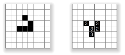
Figure 1. A glider (left) and its next generation (right).
For example, Figure 1 shows a well-known pattern called the glider composed of five live cells (left), and the resulting pattern after the B3/S23 rules are applied (right). The numbers show how many live neighbours each live cell had in the previous state.
2. Long Life
We introduce the term "Long Life" to describe a miniature 8x8 version
of the game, in which each board state is encoded as a single 64-bit
long
integer. For example the glider shown above is encoded as the following hexadecimal
number:
longstate = 0x1C10080000L;// bits describing glider
Each on-bit in this number corresponds to a live cell, as shown in Figure 2.
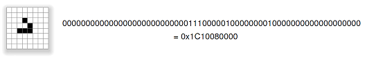
Figure 2. 64-bit encoding of a glider on the 8x8 grid.
The 8x8 grid wraps around at the edges, so that edge cells count as neighbours for the corresponding cells on opposite edges, making the grid topologically equivalent to the surface of a torus. This allows repeated cycles to occur, such as the glider's period 32 cycle shown below in Figure 3.
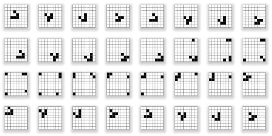
Figure 3. The 32-generation cycle of a glider in Long Life.
The glider repeats its shape every four generations. It also moves one step diagonally every four generations, which is described as a having a speed of c/4, hence the glider's cycle period on the 8x8 grid is 8x4 = 32 generations. Note that the glider wraps around the board edges to re-enter on the opposing sides, in toroidal fashion.
This version of the game is also called "Long Life" because its format came about through an investigation into creative search spaces defined by 64 bits, and the desire to seek the longest and most interesting Life cycles that can occur within this space.
We now present two algorithms for applying one generation of the B3/S23 rules to a given 64-bit state; a naïve iterative approach and a much faster bitwise-parallel approach.
3. Iterative Approach
The obvious way to calculate the next generation from a given state is to visit each cell, count its neighbours, and apply the S3/B23 rules:
	for each row
		for each column
			count live neighbours (with wraparound)
			cell' <= (count==3 or (cell==1 and count==2)) ? 1 : 0
While this is easy to express, its implementation is complicated by the need
to handle neighbours that wrap around board edges, and the fact that cell
values are encoded as bits within an integer. The following function nborCount()
returns the number of live neighbours for the cell at location [row, col],
wrapping around board edges as appropriate:
final int[][]adj= { {-1,-1}, {-1,0}, {-1,1}, {0,1}, {1,1}, {1,0}, {1,-1}, {0,-1} };intnborCount(final longstate,final introw,final intcol) {intcount = 0;for(intnbor = 0; nbor < 8; nbor++) {final intrr = (row +adj[nbor][0] +dim) %dim;final intcc = (col +adj[nbor][1] +dim) %dim; count += (state >>> (rr *dim+ cc)) & 1; }returncount; }
It's then just a matter of stepping through each cell, counting its neighbours, and turning on those bits that correspond to cells that satisfy the B3/S23 rules:
final intdim= 8;longstep(final longstate) {longresult = 0;for(introw = 0; row <dim; row++)for(intcol = 0; col <dim; col++) {final intcount = nborCount(state, row, col);final longbit = 1L << (row *dim+ col);final booleanon = (state & bit) != 0;if(count == 3 || on && count == 2) result |= bit; }returnresult; }
4. Bitwise-Parallel Approach
The above algorithm is correct and straightforward, but can be significantly improved by exploiting the single-integer representation, to perform the Life calculation over all cells at once in a bitwise-parallel manner. First, we define a mask for each set of edge cells, as shown in Figure 4:
static final longLEFT= 0x8080808080808080L;static final longRIGHT= 0x0101010101010101L;static final longTOP= 0x00000000000000FFL;static final longBOTTOM= 0xFF00000000000000L;static final longNOT_LEFT= ~LEFT;static final longNOT_RIGHT= ~RIGHT;
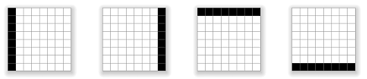
Figure 4. The four edge cell sets.
Next, we define three variables bit1, bit2 and bit3 that act as binary registers
to hold the result of the live neighbour count for each cell. This forms a
bit plane adder in which each bit position within the registers accumulates
the count for a particular grid cell:
longbit1;longbit2;longbit3;
It is not necessary to count any higher than three bits, as any sum that flows over into the third bit will represent a count of at least 22 = 4 live neighbours, which means that that cell cannot live in the next generation. For example, Figure 5 shows how the bit values are accumulated for a given cell (cell 22 in this case) to give a binary value of 110 (= 6 in decimal). Cell 22 has six live neighbours, so will not itself live in the next generation.
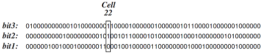
Figure 5. The count for cell 22 is binary 110, indicating six live neighbours.
The following function add() adds a neighbour value (0 or 1) to the count for each cell, and stores the result in the bit plane adder defined by bit1, bit2 and bit3, carrying values as needed. This is performed over all cells at once in a bitwise-parallel fashion, similar to Niemiec's suggestion of assigning three bits to each cell and applying a parallel adder [2]:
voidadd(final longcXX) {final longcarry1 =bit1& cXX;final longcarry2 =bit2& carry1;bit1^= cXX;bit2^= carry1;bit3|= carry2; }
The following function brings this all together by: 1) shifting the eight neighbours into position relative to input state c11, 2) accumulating neighbour counts in the three bit registers, and 3) applying a simple calculation that enforces the B3/S23 rules over all cells of the result at once:
longstep(final longc11) {// Shift neighbors into position, with wraparoundfinal longc10 = c11 >>> 8 | ((c11 &TOP) << 56);final longc12 = c11 << 8 | ((c11 &BOTTOM) >>> 56);final longc00 = (c10 &NOT_LEFT) << 1 | ((c10 &LEFT) >>> 7);final longc01 = (c11 &NOT_LEFT) << 1 | ((c11 &LEFT) >>> 7);final longc02 = (c12 &NOT_LEFT) << 1 | ((c12 &LEFT) >>> 7);final longc20 = (c10 &NOT_RIGHT) >>> 1 | ((c10 &RIGHT) << 7);final longc21 = (c11 &NOT_RIGHT) >>> 1 | ((c11 &RIGHT) << 7);final longc22 = (c12 &NOT_RIGHT) >>> 1 | ((c12 &RIGHT) << 7);// Reset the bit registersbit1= 0;bit2= 0;bit3= 0;// Accumulate live neighbor countsadd(c00); add(c01); add(c02); add(c10); add(c12); add(c20); add(c21); add(c22);// Return live casesreturn((c11 |bit1) &bit2& ~bit3); }
The input value c11 represents the unshifted cell values of the current state,
while c00... c22 represent their relative neighbours, shifted as appropriate,
as shown in Figure 6.
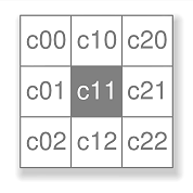
Figure 6. A cell and its eight neighbours.
After the eight neighbour values are accumulated in the bit1, bit2 and bit3 registers, then live cells in the following generation will satisfy one of the following cases:
| c11 | bit1 | bit2 | bit3 | |||
| 0 | 1 | 1 | 0 | // dead with 3 live neighbours |
||
| 1 | 0 | 1 | 0 | // live with 2 live neighbours |
||
| 1 | 1 | 1 | 0 | // live with 3 live neighbours |
These cases, and only these cases, are given by:
(c11 |bit1) &bit2& ~bit3
5. Comparison
The iterative algorithm performs around 7,000 binary operations (ops) per generation - those nested loops do add up! - while the bitwise-parallel algorithm performs 82 ops per generation in the format shown above. A slightly optimised version of this code performs 71 ops per generation.
The iterative algorithm performs around 15,000 generations per second on a single thread of a standard MacBook laptop with i5 processor, while the bitwise-parallel method performs over 1,500,000 generations per second. This approximately 100 times speed-up is important when searching for interesting cyclic patterns, as such patterns are few and far between, and many generations must be calculated to test each one.
In terms of computational complexity, the iterative approach is ostensibly polynomial time due to its nested loops while the bitwise-parallel approach is constant time. However, this analysis should be taken with a grain of salt, as the data sizes involved are small and are in fact constant - the grid will always be 8x8 and the each cell will always have eight neighbours - so the performance comparisons given above are more meaningful.
The fast bitwise-parallel algorithm was devised by the second author, based on his earlier Fast Life algorithm for the Life Flow iPad app [3]. The Fast Life algorithm uses the triple-bit register approach to process entire rows at once in a bitwise-parallel manner, and applies to grids larger than 8x8. The Long Life algorithm shown here is the next step in efficiency, as it exploits the single integer representation to process the entire grid at once rather than row-by-row.
Other fast bitwise approaches for the Game of Life include those by Niemiec [2], Pepicelli [4], Hansel [5], Finch [6] and Cherniavsky [7], although none of these describe a method tailored to a single data type that processes the entire grid at once with wraparound. Our approach has potential application to an analogue implementation of the game for an 8x8 LED matrix, which has recently become a popular exercise for electronics students and hobbyists [8].
Complete Java code for the Long Life algorithm described in this article
can be found at:
http://www.cameronius.com/research/LongLife.java
6. Conclusion
This article shows how the representation of a problem can have a profound effect on its implementation. Choosing an appropriate representation, i.e. 64-bits encoded as a single long integer, allows an algorithmic improvement that performs around 100 times fewer operations than an iterative approach to yield a 100 times speed-up, a greater improvement than is typically achieved with the incremental optimisation of code. This demonstrates the power of lateral thinking - literally in this case, as the bit plane adders that count live neighbours are orthogonal to the data types that they are adding.
References
[1] Gardner, M. (1970) "The fantastic combinations of John Conway's new solitaire game 'life'", Scientific American, 223, October, 120-123.
[2] Niemiec, M. (1979) "Life Algorithms", BYTE, January, 90-97.
[3] Browne, C. (2010) Life Flow, iPad app, https://itunes.apple.com/us/app/life-flow-for-ipad/id365729200?mt=8.
[4] Pepicelli, G. (2005) "Bitwise Optimization in Java: Bitfields, Bitboards, and Beyond", http://onjava.com/pub/a/onjava/2005/02/02/bitsets.html.
[5] Hensel, A. (1999) "About my Conway's Game of Life Applet", http://www.ibiblio.org/lifepatterns/lifeapplet.html.
[6] Finch, T. (2003) "An Implementation of Conway's Game of Life", http://dotat.at/prog/life/life.html.
[7] Cherniavsky, B. (2003) "BitLife - A Bitwise Stack of Life Games", http://bitlife.sourceforge.net.
[8] Ian (2010) "Arduino Game of Life on 8x8 LED Matrix", http://brownsofa.org/blog/archives/170.
Appendix: Java Code Listing for the Long Life Algorithm
// Edge cell masksstatic final longLEFT= 0x8080808080808080L;static final longRIGHT= 0x0101010101010101L;static final longTOP= 0x00000000000000FFL;static final longBOTTOM= 0xFF00000000000000L;static final longNOT_LEFT= ~LEFT;static final longNOT_RIGHT= ~RIGHT;// Registers for bit plane adderlongbit1;longbit2;longbit3;// Add the count for neighbour cXX to the bit registersvoidadd(final longcXX) {final longcarry1 =bit1& cXX;final longcarry2 =bit2& carry1;bit1^= cXX;bit2^= carry1;bit3|= carry2; }// Perform one step of the B3/S23 rules to state c11longstep(final longc11) {// Shift neighbors into position, with wraparoundfinal longc10 = c11 >>> 8 | ((c11 &TOP) << 56);final longc12 = c11 << 8 | ((c11 &BOTTOM) >>> 56);final longc00 = (c10 &NOT_LEFT) << 1 | ((c10 &LEFT) >>> 7);final longc01 = (c11 &NOT_LEFT) << 1 | ((c11 &LEFT) >>> 7);final longc02 = (c12 &NOT_LEFT) << 1 | ((c12 &LEFT) >>> 7);final longc20 = (c10 &NOT_RIGHT) >>> 1 | ((c10 &RIGHT) << 7);final longc21 = (c11 &NOT_RIGHT) >>> 1 | ((c11 &RIGHT) << 7);final longc22 = (c12 &NOT_RIGHT) >>> 1 | ((c12 &RIGHT) << 7);// Reset the bit registersbit1= 0;bit2= 0;bit3= 0;// Accumulate live neighbor countsadd(c00); add(c01); add(c02); add(c10); add(c12); add(c20); add(c21); add(c22);// Return live casesreturn((c11 |bit1) &bit2& ~bit3); }
Cameron Browne and Stephen Tavener - Imperial College London - March 2013